The Calculation Of Probabilistic Seismic Hazard Analysis (psha)
Seismic hazard analysis is a method used to assess the potential ground shaking caused by earthquakes, considering various seismic source models, magnitudes, distances, and depths. This assessment relies on ground motion prediction equations (GMPEs) to estimate shaking intensity. One widely used approach is Probabilistic Seismic Hazard Analysis (PSHA), which evaluates the likelihood of different levels of ground shaking occurring over a given time period.
The primary objective of PSHA is to estimate the annual frequencies of exceedence for various intensity measures (IM), such as Peak Ground Acceleration (PGA) and Spectral Acceleration (SA (T)). The result of this analysis is typically represented as a hazard curve, which shows the annual frequency of exceeding different levels of ground motion intensity. This approach helps in understanding seismic risk and is essential for earthquake-resistant design, land-use planning, and risk mitigation strategies. This method was introduced by Cornell, 1968. Then, McGuire, 2004 has developed more comprehensive of this method.
The PSHA has four steps to be analysed:
- Identification and characterization of seismic source models
- Estimation of earthquake occurrence model through the magnitude-frequency distribution
- Calculation of ground motion for all possible magnitudes and distances
- Probability calculation
We will explain for each setp above.
1. Seismic Source Models Identification
The first step in PSHA is the identification and characterization of seismic sources, also known as source zones, earthquake sources, seismic seismic zones or seismic source models, that could potentially affect the site of interest. These sources can be classified into three main types:
- Area Sources – Used when specific faults cannot be identified, representing regions where earthquakes are assumed to occur with uniform probability.
- Fault Sources – Defined based on known geological faults, where earthquake ruptures are expected to occur along fault lines.
- Point Sources – Represent localized seismic activity, often used for isolated events or regions with sparse seismic data.
In classical PSHA, seismicity within each source zone is often assumed to follow a uniform distribution, meaning earthquakes are equally likely to occur at any point within the defined area. By combining the earthquake occurrence probability distributions with the spatial extent of the sources, PSHA generates distributions for earthquake magnitude, location, and recurrence over time. Ultimately, a seismic source model can be viewed as a set of possible earthquake scenarios, each characterized by a specific magnitude, location, and seismic activity rate, which are essential inputs for estimating ground motion probabilities at a given site.
2. Earthquake Occurrence Model Estimation
Next, the earthquake occurrence model in terms of frequency-magnitude is estimated for each seismic source model. The model is assumed as Poisson distribution in time domain randomly. It explains that the future earthquake does not depend on the the past earthquake. The general model to describe the earthquake occurrence is Gutenberg-Richter relationship and it is also called as earthquake magnitude recurrence model as written in Equation 1,
\[log_{10} N = a - bM\]where the \(N\) is the number of earthquakes or rate of earthquakes, \(M\) is the magnitude (it can refer to magnitude of completeness, \(M_c\)), \(a\) is the seismicity rate, and \(b\) is the ratio between the number of small and large earthquakes. This relationship is interpreted as a cumulative relationship of number of earthquakes with magnitude equal or greater than \(M\). The \(a\) and \(b\) values can be estimated by using either linear regression or Maximum-Likelihood method (Aki, 1965) as written in Equation 2
Maximum-Likelihood Estimation
\[b = \frac {log_{10} e} {\bar M - M_c}\]where \(\bar M\) is the magnitude average and for the estimation variance of b-value can be estimated by using \(b_{std} = \frac {b} {\sqrt N}\). Then the Shi and Bolt, 1982 formulated another approach to estimate the variance of b-value as Equation 3 below
\[b_{std} = 2.30 b^2 \sqrt \frac {\Sigma_{i=1}^N (M_i - \bar M)^2} {N(N-1)}\]where \(N\) is the number of earthquakes. The a-value is simple estimated by using Equation 4
\[a = log_{10} N + bM\]where the \(log_{10} N\) is the number of earthquake when the \(M\) is equal to \(M_c\). All these parameters are determined by using earthquake catalog during a period of time. In general, the only mainshock (independent earthquake) is considered for this analysis.
3. Ground Motion Calculation
Furthermore, the calculation of ground motion and its uncertainty. This calculation make uses of a empirical equation which is called as Ground Motion Prediction Equations (GMPEs) (source 1, source 2). This approach is to estimate a potential ground motion level given by magnitude, type of source model, local site effect (\(V_s30\)), and distance from source to certain location. The ground motion level is represented as Peak Ground Acceleration (PGA), Peak Ground Velocity (PGV), Peak Ground Displacement (PGD), and Spectral Acceleration (SA).
For an example, we use the GMPE of Fukushima and Tanaka, 1990 as Equation 5 below
\[log_{10} A = aM_w - log_{10}(R + c10^{aM_w}) - bR + d\]where \(A\) is in \(cm/s^2\), \(M_W\) is moment magnitude, \(R\) is the distance between source to a site, \(a=0.42\), \(b=0.0033\), \(c=0.025\), \(d=1.22\), and \(\sigma=0.28\) (standard deviation).
If we have a certain earthquake at a certain hypocenter (\(lon_{hypo}\), \(lat_{hypo}\), and \(depth\)) with a certain \(M_w\), then we can estimate a ground motion level in a particular site (\(lon_{site}\) and \(lat_{site}\)) with a ditance \(R\) from the hypocenter.
4. Probability Calculation
The aim of PSHA is for estimating annual rate of exceedance given an magnitude of event \(m\) from a number of sources \(n_S\) to a particular location with distance \(r\) in terms of a intensity measure \(IM\) will exceeds a particular value \(y\), \(\lambda (IM > y)\), as written in Equation 6a below
\[\lambda (IM > y) = \Sigma_{i=1}^{n_s} \lambda (M_i > m_{min}) \int_{m_{min}}^{m_{max}} \int_{R|M} P[IM \ge y | m, r] f_M (m) f_{R|M} (r|m) dr dm\]The Equation 6a above can be written in discrete form as shown in the Equation 6b below
\[\lambda (IM > y) = \Sigma_{i=1}^{n_s} \lambda (M_i > m_{min}) \Sigma_{j=1}^{n_m} \Sigma_{k=1}^{n_r} P[IM \ge y | m_j, r_k] P(M_i = m_j) P(R_i = r_k)\]The
\[P[IM \ge y | m, r]\]is the probability of the \(IM\) will exceeds a particular value \(y\) for given magnitude \(m\) and distance \(r\).
The \(IM\) can be PGA or SA at any period and \(y\) is the ground motion value. This is calculated by using Equation 7 below
\[P[IM \ge y | m, r] = 1 - \phi (\frac {\ln y - \overline {\ln IM}} {\sigma_{\ln IM}})\]where the \(\phi()\) is a normal cumulative distribution function, \(\overline {\ln IM}\) is a median of ground motion (estimated from GMPE), and \(\sigma_{\ln IM}\) is a standard deviation of ground motion. We can also calculate the probability of ground motion at certain intensity level by using the equation below
\[P(IM = y_i) = P(IM > y_i) - P(IM > y_{i+1})\]The \(P(M = m_j)\) is the probability of occurrence of a series of magnitudes and calculated by using Equation 8
\[P(M = m_j) = F_M (m_{j+1}) - F_M (m_j)\]and the \(F_M(m_j)\) is the magnitude cumulative distribution function (CDF) that can be calculated by using Equation 9a
\[F_M(m_j) = 1 - 10^{-b (m_j - m_{min})}\]if the magnitude maximum \(m_{max}\) is identified, then the equation become Equation 9b below
\[F_M(m_j) = \frac {1 - 10^{-b (m_j - m_{min})}} {1 - 10^{-b (m_{max} - m_{min})}}\]The \(P(R = r_k)\) is the probability of occurrence of series of distances. It is calculated by using
\[P(R = r_k) = F_R (r_{k+1}) - F_R (r_k)\]where the \(F_R(r_k)\) is the cumulatif distribution function (CDF) of distance. This is estimated by depending on the type of source geometry, such as area or simple fault line source. If the distance \(R\) is equal to the fixed value then the \(P(R = r_k)\) is equal to 1.
The equation 6b is the foundation for PSHA calculation and hazard curve is the product.
5. Examples
5.1. Example 1: A single magnitude, certain distance, and single intensity measure value
Suppose we want to estimate the annual rate of exceedence greater than and equal to 0.1 g given \(M_w = 6\) at a certain point with a distance 10 Km from a simple fault source. The fault has occurrence rate (\(\lambda\)) of 0.01 per year. We can calculate this by the follwoing steps:
1. GMPE Calculation We use the GMPE of Fukushima and Tanaka, 1990 as Equation below
\[log_{10} A = aM_w - log_{10}(R + c10^{aM_w}) - bR + d\]where \(A\) is in \(cm/s^2\), \(M_W\) is moment magnitude, \(R\) is the distance between source to a site in Km, \(a=0.42\), \(b=0.0033\), \(c=0.025\), \(d=1.22\), and \(\sigma_{log_{10} A}=0.28\) (standard deviation).
\[log_{10} A = 0.42 * 6 - log_{10} (10 + 0.025*10^{0.42 * 6}) - 0.0033*10 +1.22 = 2.44\]\(A = 278.65 cm/s^2\) or equal to \(0.3 g\)
2. Calculationg the CDF of GMPE Using the Equation 7 to calculate the probability of the ground motion that exceed 0.1 g
\[P[PGA \ge 0.1 g | m=6, r=10] = 1 - \phi (\frac {\ln (0.1) - \ln (0.3)} {0.28}) = 0.76\]3. Estimating CDF of Magnitude and Distance Since we use the single magnitude and distance, the CDF of magnitude, P(M=m) is equal to 1 as well as CDF of distance, then
\(P(M=6) = 1\) and \(P(R = 10) = 1\)
4. Substituting to The Main Equation All the above parameters are substituted into the following equation, since we only consider for one source, the sigma of the source is ignored.
\(\lambda (PGA > y) = \lambda P[PGA \ge y | m, r] P(M= m) P(R = r)\) \(\lambda (PGA > 0.1 g) = \lambda P[PGA \ge 0.1 g | 6, 10] P(M= 6) P(R = 10)\) \(\lambda (PGA > 0.1 g) = 0.01 * 0.76 * 1 * 1 = 0.0076\)
So, for the earthquake magnitude of 6 on the site 10 Km from the fault will exceed the ground motion greater than 0.1 g at annual rate of 0.0076 per year.
Here is the Python code for the above calculaiton
import numpy as np
from scipy import stats

rate = 0.01  # rate of a simple fault per year
r = 10  # distance in KM
M = 6  # magnitude
im = 0.1  # PGA in g

# coefficients of GMPE
a,b,c,d = 0.42,0.0033,0.025,1.22
std = 0.28  # std log10_A

# Calculating the ground motion given a magnitude and distance
"""
GMPE: Fukushima and Tanaka, 1990
(https://iisee.kenken.go.jp/eqflow/reference/1_10.htm)
"""
lnA = a*M - np.log10(r + c*10**(a*M)) - b*r + d
A = 10**lnA # in cm/s^2
A_in_g = A / 918  # converting to g

# calculating the probability of ground motion that exceed to 0.1 g
prob_gm = 1 - stats.norm.cdf(im, loc=A_in_g, scale=std)

# calculating the annual rate of exceedence
PM, PR = 1, 1
annual_rate = rate * prob_gm * PM * PR

print(f"Ground motion in original unit: {A:.2f} cm/s^2")
print(f"Ground motion in g unit: {A_in_g:.2f} g")
print(f"P[PGa > {im} g]: {prob_gm:.2f}")
print(f"Annual rate: {annual_rate:.4f} per year")
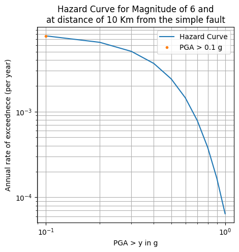
5.2. Example 2: A single magnitude, certain distance, and a series intensity measure values
Suppose we want to estimate the annual rate of exceedence for intensity measure from 0.1g until 1 g given \(M_w = 6\) at a certain point with a distance 10 Km from a simple fault source. The fault has occurrence rate (\(\lambda\)) of 0.01 per year. We use the same process as the Example 1 above for each intensity value. We can use the simple Python program code for the calculation simulatinously as shown in the box below.
"""
Calculating the annual rate of exceedance for a series of intensity measure
"""
import numpy as np
from scipy import stats
import matplotlib.pyplot as plt
import pandas as pd

rate = 0.01  # rate of a simple fault per year
r = 10  # distance in KM
M = 6  # magnitude

# Defining the series of intensity measure
im = np.arange(0.1,  1.1,  0.1)

# coefficients of GMPE
a,b,c,d = 0.42,0.0033,0.025,1.22
std = 0.28  # std log10_A

# Calculating the ground motion given a magnitude and distance
"""
GMPE: Fukushima and Tanaka, 1990
(https://iisee.kenken.go.jp/eqflow/reference/1_10.htm)
"""
lnA = a*M - np.log10(r + c*10**(a*M)) - b*r + d
A = 10**lnA # in cm/s^2
A_in_g = A / 918  # converting to g

# calculating the probability of the series ground motion that exceed for each value
prob_gm = 1 - stats.norm.cdf(im, loc=A_in_g, scale=std)

# calculating the annual rate of exceedence
PM, PR = 1,  1
annual_rates = rate * prob_gm * PM * PR

# collect data
data_hc = pd.DataFrame({
	"PGA": im,
	"annual_rate": annual_rates
})

# calculating the probability at certain ground motion level
prob_gm_at_y = list()
for i in  range(len(prob_gm)-1):
prob_gm_at_y.append(prob_gm[i] - prob_gm[i+1])

prob_gm_at_y = np.array(prob_gm_at_y)

# Plot the hazard curve
fig, ax = plt.subplots(figsize=(5,5))
ax.loglog(im, annual_rates, label='Hazard Curve')
ax.loglog(single_im, annual_rate,  '.', label=f'PGA > {single_im} g')
ax.grid(which="both")
ax.set_axisbelow(True)
ax.set_xlabel("PGA > y in g")
ax.set_ylabel("Annual rate of exceednece (per year)")
ax.set_title(f"Hazard Curve for Magnitude of {M} and\nat distance of {r} Km from the simple fault")
plt.legend()
plt.show()
The above program will show the hazard curve as below
Reference
- Baker, J. W., Bradley, B. A., and Stafford, P. J. (2021). Seismic Hazard and Risk Analysis. Cambridge University Press, Cambridge, England.
- Baker, J. W., Bradley, B. A., and Stafford, P. J. (2008). An Introduction to Probabilistic Seismic Hazrad Analysis
- C. Allin Cornell; Engineering seismic risk analysis. Bulletin of the Seismological Society of America 1968;; 58 (5): 1583–1606. doi: https://doi.org/10.1785/BSSA0580051583
- McGuire. (2004) Seismic Hazard and Risk Analysis. Monograoh Series. Earthquake Engineering Research Institute